Lab Six

Preliminaries

Last week, we built a spreadsheet that compared the cost of purchasing 3 different cars based on purchase price, interest, and insurance. In this lab, we will add much more significant detail to analyze and compare the cost of ownership of three different vehicles over 4 years. This analysis is based on certain assumptions.

This lab will demonstrate that there is more to consider when purchasing a vehicle than just the purchase price. It will show you how to analyze this data.

Goals

1. Using Microsoft Excel
2. Translate a word problem to an Excel Spreadsheet
3. Do What-if analysis

To Do

1. Start Microsoft Excel

Open the file you created last week. Click file, open, A:\, file name.

2. How choose which car to purchased?

Saturn The manufacturer estimates that this vehicle gets 37 miles per gallon of gasoline. Normal service and maintenance charges are estimated to be $.02 per mile. The vehicle has a 36000-mile unlimited bumper to bumper warranty. 

Toyota RavThe manufacturer estimates that this vehicle gets 38 miles per gallon of gasoline. Normal service and maintenance charges are estimated to be $.06 per mile. The vehicle has a 70,000-mile unlimited bumper to bumper warranty.

Ford Escape The manufacturer estimates that this vehicle gets 34 miles per gallon of gasoline. Normal service and maintenance charges are estimated to be $.03 per mile. The vehicle has a 60,000-mile unlimited bumper to bumper warranty.

Assumptions

You are going to analyze the total cost of owning each vehicle over a four-year period.

The cost of fuel for the first year is 1.429 per gallon and it will increase 5 percent each year. 

Last year you drove 30,000 miles. You expect to drive the same in each of the four years under analysis.

For every 20,000 miles driven that exceeds the warranty, you can expect a $225 repair bill. For example, the repair bills for the Toyota will be (((4*30,000)-70,000)/20,000)*225. 

1. Create a spreadsheet to compare the total cost over four years of these three vehicles. The vehicles should be in the columns and the expenses in the rows.

 

 
 
 


The following items should be Assumptions.

• Assumptions MUST only appear once!!!!!. They MUST be addressed using absolute addressing. If assumptions appear more than once in your spreadsheet and are not addressed using absolute addressing, you will be severely penalized.
• The word Assumptions should appear in row 4 column A with font size 12.
• Beginning with row 5, the name of the item should appear in column A and the value in Column B.
• Assumption: The cost of fuel.
• Assumption: The percentage increase per year of the cost of fuel
• Assumption: The miles per year 
• Assumption: Cost of the repair each repair bill over warranty
• Assumption: Miles exceeding warranty that will result in a repair bill
2. Calculate the total cost of ownership for over four years for each of the three vehicles. 
• Before listing the expenses, you need to list some items. These items should begin in row 20 (leaving row 19 blank). These items include: miles of waranty, service and mantenance per mile, miles per gallon, and gallons per year.

 

 
 
 
 
 

Note, row 23, gallons per year, should be a formula that references the miles driven per year absolutely and miles per gallon relatively. Remember the rules of algebra, the units must work out. 

• Rows 24, 25, 26, and 27 should contain formulas for the cost of fuel for year 1, year 2, year 3, and year 4 respectively.
• Row 28 should contain a formula for the cost of maintenance.
• Row 29 should contain a formula for the cost of repairs.
• Leave row 30 blank and row 31 should contain the total cost of ownership for each vehicle over 4 years. You should label the row and the label should be font size 14 and bold.
• When making ALL calculations, you must properly reference assumptions and data stored in worksheet cells. You must not type in values. For example, percent increase in fuel is entered once in the assumptions. In calculating the fuel cost for years 2, 3, and 4, you must reference this assumption, not hard code in values.
• Be sure to use relative and absolute references where appropriate. When referencing the items in the assumptions, you MUST use absolute references. When referencing a value specific to a vehicle (e.g. miles of warranty), you must use relative references.
• By using proper relative and absolute references, formulas only have to be entered for the first vehicle and can be copied to the other two.
• Cells must be properly formatted. Cells containing dollar amounts should be formatted as currency and all others should be general. Click on Format on the main menu, then cells and make the appropriate choice. 
• Row 34 Column G should contain the label Least expensive. Enter a formula into Column F to determine the minimum of Column's C-E of Row 31.
• Row 35 Column G should contain the label Most expensive. Enter a formula into Column F to determine the maximum of Column's C-E of Row 31.
Be sure to verify that the data you have entered is correct. Be sure to verify that ALL of the formulas that you have entered are correct. Remember, Garbage In Garbage Out .
3. Print out your worksheet.
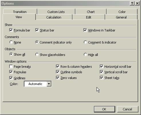
4. Print your worksheet showing the formulas instead of the results. The way you do this is to click on tools, then options, and select the Window options tab. On the Windows options, check the formulas box. Then click ok. This will change the worksheet to display your formulas instead of the results of their calculation. Print out the worksheet in this format. You can then click on tools, then options, and select Window options tab. Remove the check and click ok to set the display back to displaing results. NOTE: in order to get credit for this lab, the spreadsheet must be making ALL calculations. 
5. Add a 3-D column chart to the worksheet as described in class. Print the results. The 3-D chart should appear under your totals.

 

 
 
 
 
 

Remember, to create 3-D chart, Select the area to be in the chart. This should include price plus interest, fuel cost, Insurance, maintenance, and repair. Click on the Chart Wizard button. With column selected in the Chart type list, Click the 3-D column chart sub-type (column 1, row 2 n the chart sub-type area. Poin to finish and click. You can then drag the chart to the appropriate place.

6. Save your worksheet on diskette.
7. Do what if analysis.
• Increase the miles per year to 35,000.
• Increase the starting fuel price to 1.529
• Increase the percent increase in fuel price to 6 percent
• Print the results
8. Which car would you buy? After examining your initial spreadsheet and your "what if" spreadsheet, make a decision as to which vehicle you'd buy. Type this in at the bottom of your spreadsheet. Print this final result.

3. Save your spreadsheet onto your diskette

4. Hand In

Maintained by Barbara Bracken
Last Modified 11/19/2003

This page is copyright protected © by Barbara Bracken