Download and read the Excel documentation provided. Some important information is repeated below.
A cell address is made up of a column letter and a row number.
Relative Cell Address: A relative cell address is relative to the current position. When replicated, it changes relative to the new position. Relative addresses are used when the same formula applies to multiple cells operating on data relative to the cells. e.g. A3
Absolute Cell Address: Absolute cell addresses to not change when replicated. Absolute addresses are used for assumptions. e.g. $A$3, A$3, $A3
Multiple Worksheets: Excel workbooks are made up of multiple worksheets. A formula in one worksheet can address cells in other worksheets. The reference to cell in another worksheet can be absolute or relative. To address a cell in another worksheet:
sheet1!A3
sheet2!$A$3
Subaru!b5 (if the sheet has been given a name
A function performs a predetermined set of operations. Functions take parameters and return a result. Parameters are enclosed in parenthesis and separated by commas. The parameter list is specific to a function.
This lab uses seven built-in functions:
The vlookup built-in function searches for a value in the leftmost column of a table, and then returns a value in the same row from a column you specify in the table.
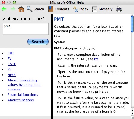
We will only be using rate, nper, and pv. fv is the balance you want to remain at the end of the term. A balance of 0 is the default, so it may be omitted. Type indicates when the payment is due. By omitting it, the default is due at the beginning of the period.

We will only be using rate, per, nper, and pv.
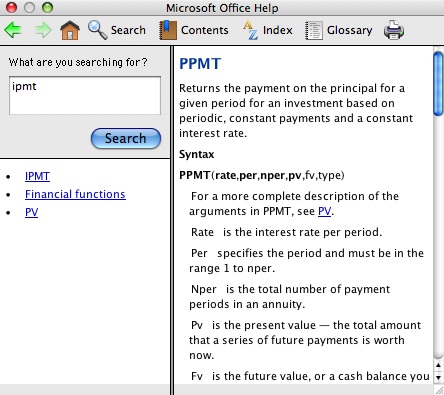
We will only be using rate, per, nper, and pv.
You will be given loan terms and the purchase price for 2 different vehicles. You will create a worksheet for each vehicle to amortize the loan for each of the vehicles. These worksheets will be used in Part 2 of this lab to calculate the total cost of ownership of the 2 different vehicles.
You are going to purchase a new vehicle. You are looking at 2 different SUV's:
The purchase price of the Subaru Outback is $29,999. The term of the car loan is 4 years, 5.125% interest.
The purchase price of the Toyota RAV4 is $26,500. The term of the car loan is 4 years, 6.275% interest.
Important note: If your formula results in ######### in the cell, all it means is that the column is not wide enough for the data. Simply widen the column. This can be done by dragging the column border to the right.
By default, excel provides 3 worksheets. When you open a new workbook, f you look at the bottom of your workbook, you should see tabs "sheet1", "sheet2", and "sheet3". The sheet names were changed in the template to "Cost of Ownership", "Subaru", and "Toyota". We will be using "Total Cost of Ownership" in the automotive lab where we will be comparing the cost of ownership of the 2 vehicles over 5 years. In the other two sheets, we are going to create the amortization tables for the Subaru and Toyota respectively.
While you will not need more than three worksheets in this lab, if you do need more than the default 3 sheets, use follow the following instructions to insert more:
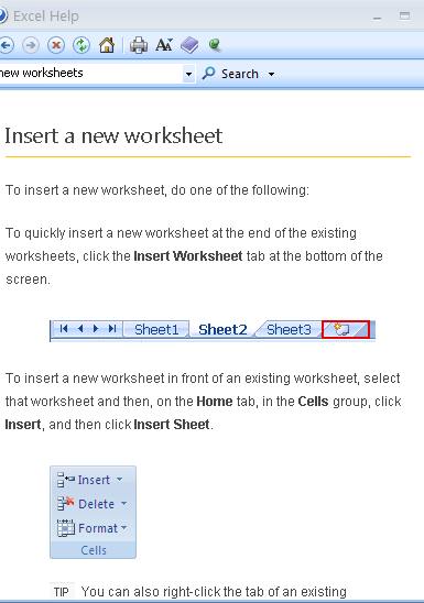
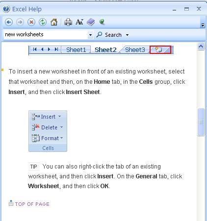
Click on the "Subaru" tab to activate sheet2.
Your name, the title, interest rate, loan term, principal, column headings, and payment numbers for the Subaru Outback have been filled in for you. Change "Your Name" to your name.
The assumptions consist of the loan information. The name of the assumption should appear in column B and the value of the assumption should appear in column C. The first assumption is in row 3. The assumptions are as follows beginning in row 3:
In C3 you are going to use the PMT built-in function to calculate the monthly payment.
The interest rate in the assumption is the annual interest rate. Therefore, in the formula you must divide the annual interest rate by 12 months as there are 12 months in a year.
The term in the assumption is the number of years of the loan. The function requires the number of payments. The term must be multiplied by 12 months per year.
The principal is an assumption.
Since the payment is a deduction, the function returns a negative value. Therefore, for purposes of this spreadsheet, the results of the formula must be negated.
Be sure to properly use absolute addressing!
The formula for payment should be:
The formula for the beginning balance for payment number 1 (B9) is going to be different than the formula for the beginning balance for payments 2-48 (B10-B56). To start with, enter the formula for payment number 1. The beginning balance comes from the assumption Principal stored in C6. The formula:
Since this formula is only going to be used in this row, it is not necessary to use absolute addressing.
C9 should contain a formula to calculate the principal portion of the payment. The PPMT built-in function is to be used.
The monthly interest rate is described under the PMT formula. The loan period is the payment number. It is obtained from $a9 (note absolute addressing for the column). See PMT for a description of the number of payments. The Principal is an assumption. Since this is a deduction, the formula should be preceded with the negative sign. This formula applies to all 48 payments.
Proper absolute and relative addressing must be used.
The formula for Cumulative Principal for Payment 1 will be different than the Formula for Cumulative Principal for Payments 2-48. The formula for Payment 1 in D9 is simply :
The Principal paid in this payment.
The IPMT built-in function is used to calculate the Interest Paid. The parameter list for IPMT is identical to the parameter list for PPMT. It should also be negated. It applies to all 48 payments. By specifying the column as absolute in the principal formula for c9 allows you to copy and paste and just change the name of the function from ppmt to ipmt.
The formula for Cumulative Interest for Payment 1 in F9 will be different than the formula for Cumulative Interest for Payments 2-48. For Cumulative Interest for Payment 1 in F9, it is simply the Interest Paid with this payment:
The formula for Paid to Date is the sum of the cumulative Principal and the cumulative Interest. This formula applies to all payments.
As a cross check, make sure that the sum in g9 equals your payment in c3.
The formula for Ending balance is the Beginning Balance minus the Principal:
This formula applies to all 48 payments.
Replicate the formulas for principal payment, C9, interest payment, E9, paid to date, G9, and ending balance, H9, from Row 9 into Row 10.
Different formulas for Beginning Balance, Cumulative Principal, and Cumulative Interest must be written for Payment Number 2 in Row 10.
The formula for Beginning Balance will come from the Ending Balance of the previous payment:
The formula for Cumulative Principal is the sum of the principal payment from this payment plus the Cumulative Principal from the previous payment:
Note the last payment the cumulative principal should equal the original principal.
The formula for cumulative Interest is similar to that of Cumulative Principal, the sum of the Interest Paid in this payment plus the Cumulative Interest from the previous payment:
Row 10 should be marked and replicated through the remainder of the 48 payments.
Check your results!!!!! At the bottom of this lab page is a link to the results. Sanity check:
You have completed a worksheet with the loan amortization for the Subaru Outback. You are now going to complete worksheet 3 with loan amortization information for the Toyota Rav4.
You must first select the data to be copied. Click in the select all entry. It is the intersection of the column
headings and the row headings. This marks the entire worksheet. Click
Edit, copy.
Click on the Sheet3 labeled Toyota at the bottom of the spreadsheet window. This will activate Sheet3.
Place the cursor in A1 of Sheet3. Click Edit Paste. This will copy the entire sheet1.
Modify the title to Toyota Rav4. Modify the assumptions appropriately.
Check your results as described under the Subaru.
Go to Sheet1 labeled Cost of Ownership.
General assumptions and per vehicle assumptions have been filled in for you in the template.
The repair costs are in a two-column table. Column A contains the total miles on the vehicle and Column B contains the estimated repair costs given the miles on the vehicle. When the vehicle has 0-15,000 miles, it is expected that there will not be any repair costs. From 15001-25000, there will be repair costs of $100, etc.
You are going to obtain the loan term, purchase price, and monthly payment from the amortization table worksheet for each vehicle. You must use absolute addressing.
In cell C24 type the formula: =Subaru!$c$5
In cell C25 type the formula: =Subaru!$c$6
In cell c26 type the formula: =Subaru!$C$3
Sanity Check: look in the last row of the amortization table for paid to date. These values should match.
Submit your completed spreadsheet via D2L.
This is © Copyright Protected by Barbara Bracken
This page is maintained by
Barbara Bracken
Last Modified
12/31/2021